dataprep: cleaning pipeline

library(dataprep)
set.seed(1)

# The size-bin columns are the ones whose names are numeric
# (1.00, 1.12, ..., 1000). This helper returns their integer
# positions, excluding the four non-size columns (`date`,
# `tconc`, `TPNC`, `monthyear`).
size_bin_cols <- function(x) {
  grep("^[-+]?[0-9]*\\.?[0-9]+$", names(x))
}

Quick start

The full data table has 7,640 rows and 65 columns: a time column, a grouping column, and 61 particle size bins. Running the full pipeline on it takes a few seconds and returns a smaller, cleaner table.

The cleaning pipeline is organised around four sequential steps, each addressing a distinct failure mode of high-resolution environmental data:

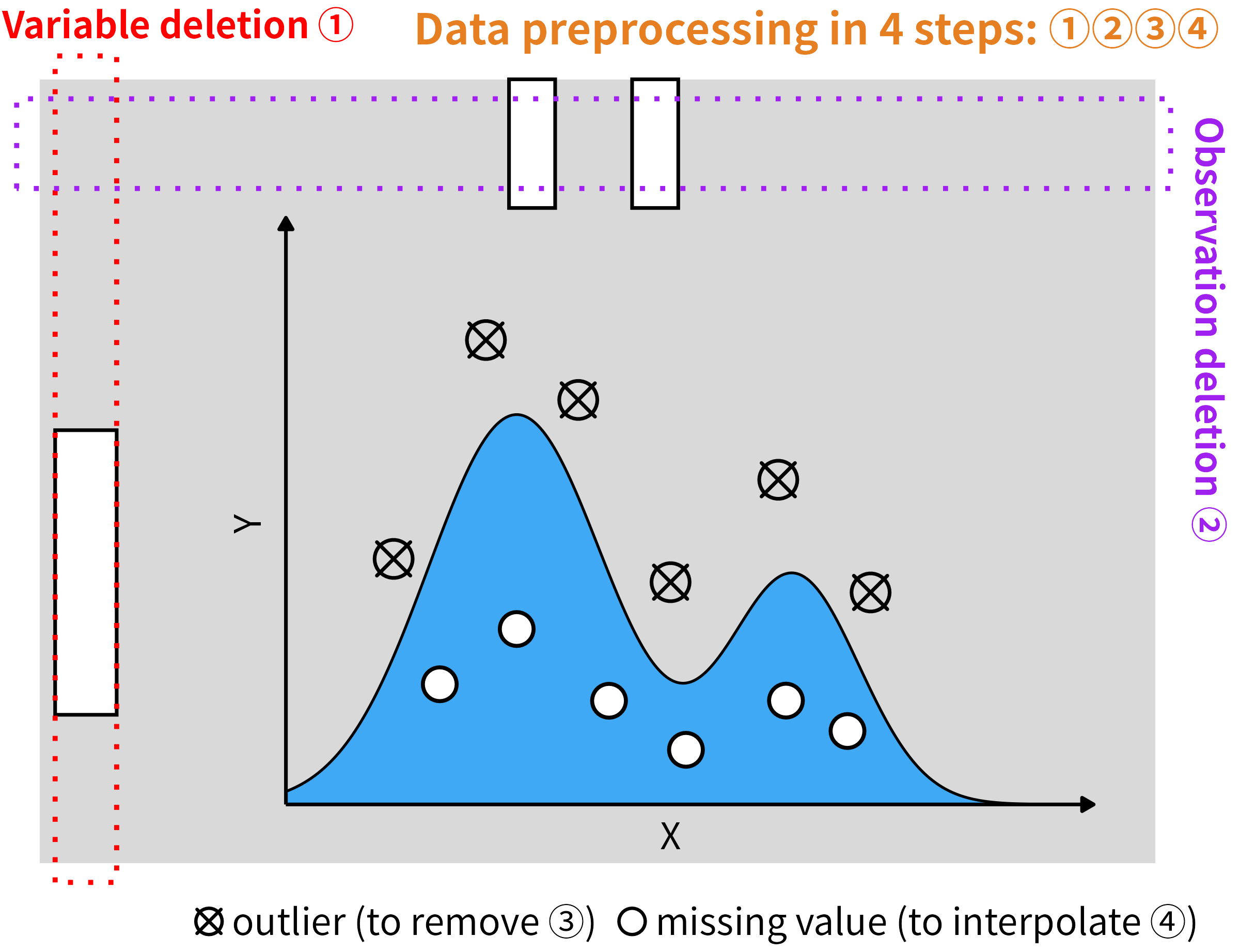
Variable deletion. Drop size bins whose missing fraction exceeds a threshold, so downstream interpolation never has to extrapolate from far-away anchors.
Observation deletion. Drop rows whose selected columns contain a consecutive missing run longer than half minutes on both sides. This guarantees every remaining point has a trustworthy anchor within half minutes.
Conditional extremum outlier removal. A single value can be a global maximum and still be legitimate, or vice versa. condextr() judges each candidate in context. Unlike a one-shot percentile cutoff, it removes fewer legitimate values and leaves no artificial outliers behind.
Short-period grouping interpolation. After steps 1–3, remaining NAs sit inside short gaps with a valid anchor within half minutes. shorvalu() interpolates within each short segment only. Interpolating across a long gap silently mixes two physically distinct regimes and can create new outliers at the segment boundary; grouping by short segments keeps the interpolation local.

cleaned <- dataprep(data,
                    cols       = size_bin_cols(data),
                    group      = 4,
                    interval   = 10,
                    times      = 10,
                    intervals  = 30,
                    cores      = 1L)
dim(cleaned)
#> [1] 6942   39

The figure below compares the top and bottom percentile curves of every size bin before and after preprocessing. The label inside each facet reports the number of observations (n) and the number of missing values (na) in that group.

percplot(
  rbind(
    transform(data[names(cleaned)],      g = "original"),
    transform(cleaned,                   g = "preprocessed")
  ),
  cols  = size_bin_cols(cleaned),
  group = ncol(cleaned) + 1
)

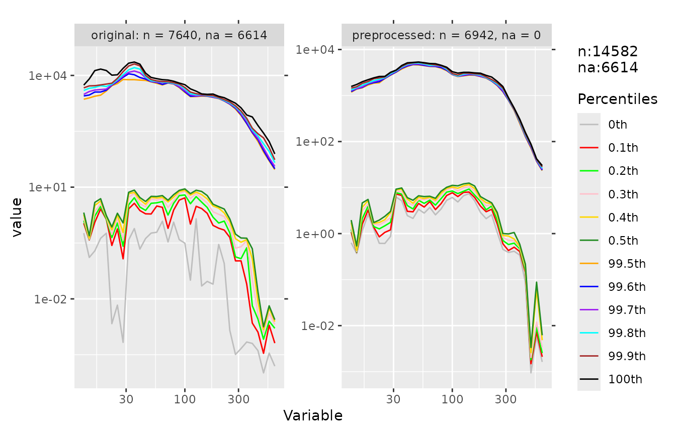
The preprocessed curves are visibly tighter: the extreme tails are shorter, the interquartile band is narrower, and the number of missing values (na) drops dramatically because whole rows with long consecutive gaps have been removed. The remaining NAs are in gaps that are too long for shorvalu to interpolate.

Note on data1. data1 is the already-aggregated seven-column version of the same dataset. It has very few missing values and no long gaps, so it is not a useful input for the cleaning pipeline. Use data for anything that modifies values; use data1 only for read-only demos (descdata, na_diagnose, percdata, percplot, descplot).

Overview

The 0.1.7 cleaning pipeline consists of four sequential steps:

Variable deletion (varidele): drop columns whose missing fraction is above a threshold.
Observation deletion (obsedele): drop rows with a run of consecutive missing values longer than half on both sides.
Outlier removal (condextr): point-by-point weighted conditional extremum; alternatives include percoutl for traditional percentile removal and detect_outliers for IQR / MAD masks.
Short-period interpolation (shorvalu): fill remaining short gaps from nearby valid values.

Steps 1–4 are wrapped by dataprep() for one-call use. Every step is designed around the same physical constraint: a valid substitute for a missing value only exists if there is an observed value within half minutes on at least one side.

Why `obsedele` changed in 0.1.7

Two behaviour changes were made in 0.1.7; both are bug fixes, but they change row counts on real data.

Change 1 — each column is scanned independently. The 0.1.5 implementation collapsed all selected columns into one long vector before computing missing runs, which merged NA runs across columns and over-deleted boundary rows. The 0.1.7 C++ backend (obsedele_cpp) scans each column separately: a row is deleted only when any selected column has a missing run longer than half minutes on both sides.

Change 2 — the boundary is inclusive. The comparison is dl <= half_seconds && dr <= half_seconds for retention, so a row whose nearest anchor is exactly half minutes away is kept. On the SMEAR I Varrio 2025 full-year dataset this retains three rows that 0.1.5 incorrectly deleted.

See vignette("dataprep-migration") for the full upgrade guide and a minimal reproduction of both changes.

The example below shows the new behaviour on a small synthetic dataset.

df <- data.frame(
  date  = as.POSIXct("2024-01-01 00:00:00", tz = "UTC") + 0:19 * 600,
  group = rep(1L, 20),
  x     = c(1, NA, NA, NA, 5, NA, NA, NA, NA, NA,
            1, NA, NA, NA, 5, NA, NA, NA, NA, NA),
  y     = c(NA, 1, NA, NA, 2, NA, NA, NA, NA, NA,
            NA, 1, NA, NA, 2, NA, NA, NA, NA, NA)
)
nrow(df)
#> [1] 20
nrow(obsedele(df, cols = c("x", "y"), group = "group", half = 2, cores = 1L))
#> [1] 2

Boundary behaviour

df_boundary <- data.frame(
  date = as.POSIXct("2024-01-01 00:00:00", tz = "UTC") + 0:4 * 600,
  x    = c(1, NA, NA, NA, 5)   # anchors at 0 and 40 minutes
)
nrow(obsedele(df_boundary, cols = "x", half = 30, cores = 1L))
#> [1] 5

All five rows survive: the two interior rows are 10 and 20 minutes from the nearest anchor, and the middle row is exactly 30 minutes (= half) — which is now treated as “within half minutes”.

`condextr` vs `percoutl`

percoutl() is a single-pass percentile threshold: every value above the top quantile or below the bottom quantile is set to NA. It is fast but has no notion of magnitude.

condextr() adds two safeguards: a percentile error margin (top.error, bottom.error) and a magnitude margin (top.magnitude, bottom.magnitude). Only the extreme point of a window is removed if it exceeds the combined threshold. This preserves a wider dynamic range while still removing the most extreme values.

The figure below illustrates the difference. The left panel shows the same series processed by the traditional percentile rule (green) and by the conditional-extremum rule (orange). The right panels show the consequences step by step: the traditional rule clips legitimate values at both ends of the distribution and then produces new outliers at the boundary between observed and interpolated points. The conditional-extremum rule removes only the extreme point of each window and leaves no artificial outlier behind.

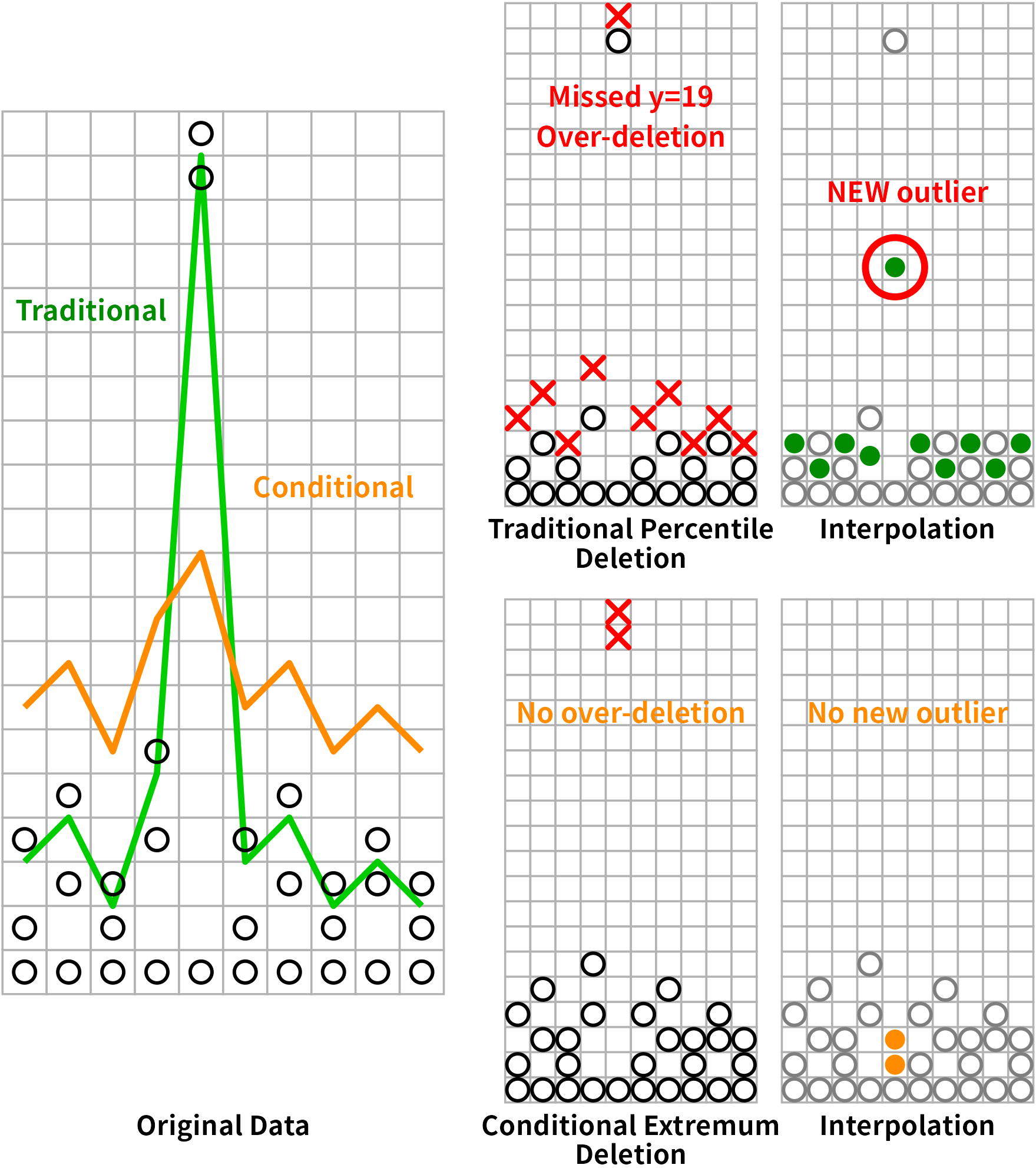
In short:

percoutl is a one-shot, unsupervised cutoff: over-deletion of legitimate values and creation of new outliers are both possible.
condextr is a per-point, context-aware rule: it removes fewer values, and the values that remain still span the original dynamic range.

Why `obsedele` is re-applied after `condextr`

condextr() sets outliers to NA. Those new NAs can join pre-existing ones and form longer missing runs than the input ever had. If the pipeline moved directly from outlier removal to interpolation, shorvalu() would silently bridge those extended gaps.

For this reason, dataprep() runs obsedele() once more after every round of outlier marking. The condextr loop is structured as:

for round in 1..times:
    for i in 1..interval:
        condextr: mark outliers in every column
    obsedele: delete rows whose NA runs now exceed half

interval controls how aggressively condextr marks points between two deletion rounds; times controls how many rounds the loop runs. Together they give the user control over the trade-off between outlier sensitivity and sample retention. optisolu() can search over this grid automatically when a percoutl reference is available.

Step-by-step walkthrough

The pipeline can also be run step by step. We use rows 3,000 to 4,000 of data — a window of about seven days that happens to span a month boundary — to keep the vignette fast and to make the group-wise behaviour visible.

data_slice <- data[3000:4000, ]

# Select the size-bin columns by name pattern: the ones whose
# names are numeric (1.00, 1.12, ... 1000). This excludes the
# four non-size columns (`date`, `tconc`, `TPNC`, `monthyear`),
# including `tconc` and `TPNC` which are numeric but not size
# bins.
num_cols_raw <- size_bin_cols(data_slice)

# Some size bins are entirely NA in this slice and must be dropped
# before any further step.
na_frac <- sapply(data_slice[, num_cols_raw], function(x) mean(is.na(x)))
table(na_frac == 1)
#> 
#> FALSE  TRUE 
#>    49    12

Step 1 — Variable deletion

varidele() drops any size bin whose missing fraction exceeds fraction. This is what removes the all-NA columns before they contaminate downstream steps.

step0 <- varidele(data_slice,
                  cols     = num_cols_raw,
                  fraction = 0.5)
num_cols <- size_bin_cols(step0)
length(num_cols)          # number of bins that survived
#> [1] 43

Step 2 — Observation deletion

step1 <- obsedele(step0, cols = num_cols, group = 4, cores = 1L)
nrow(step1)
#> [1] 772

Rows whose selected bins contain a gap longer than half minutes on both sides are removed. Every surviving row has a valid anchor within half minutes on at least one side of every missing run.

Before cleaning

percplot(step0, cols = num_cols, group = 4)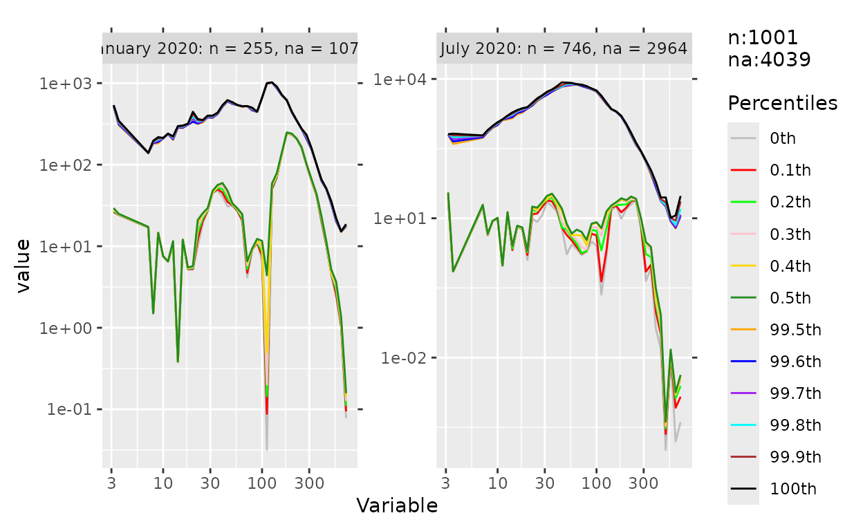

Long, flat tails at the low and high end of the size distribution indicate the presence of outliers and long stretches of missing data.

Step 3 — Conditional extremum outlier removal

step2 <- condextr(step1, cols = num_cols, group = 4,
                  interval = 10, times = 10, cores = 1L)
nrow(step2)
#> [1] 767

condextr combines a percentile threshold with an error margin and a magnitude margin, and removes only the single most extreme value in each window. Unlike percoutl, it does not flatten the tails.

Note that condextr() internally re-applies observation deletion after each round of marking. This is why the row count changes by more than just the number of NAs introduced by outlier marking alone.

After cleaning

percplot(step2, cols = num_cols, group = 4)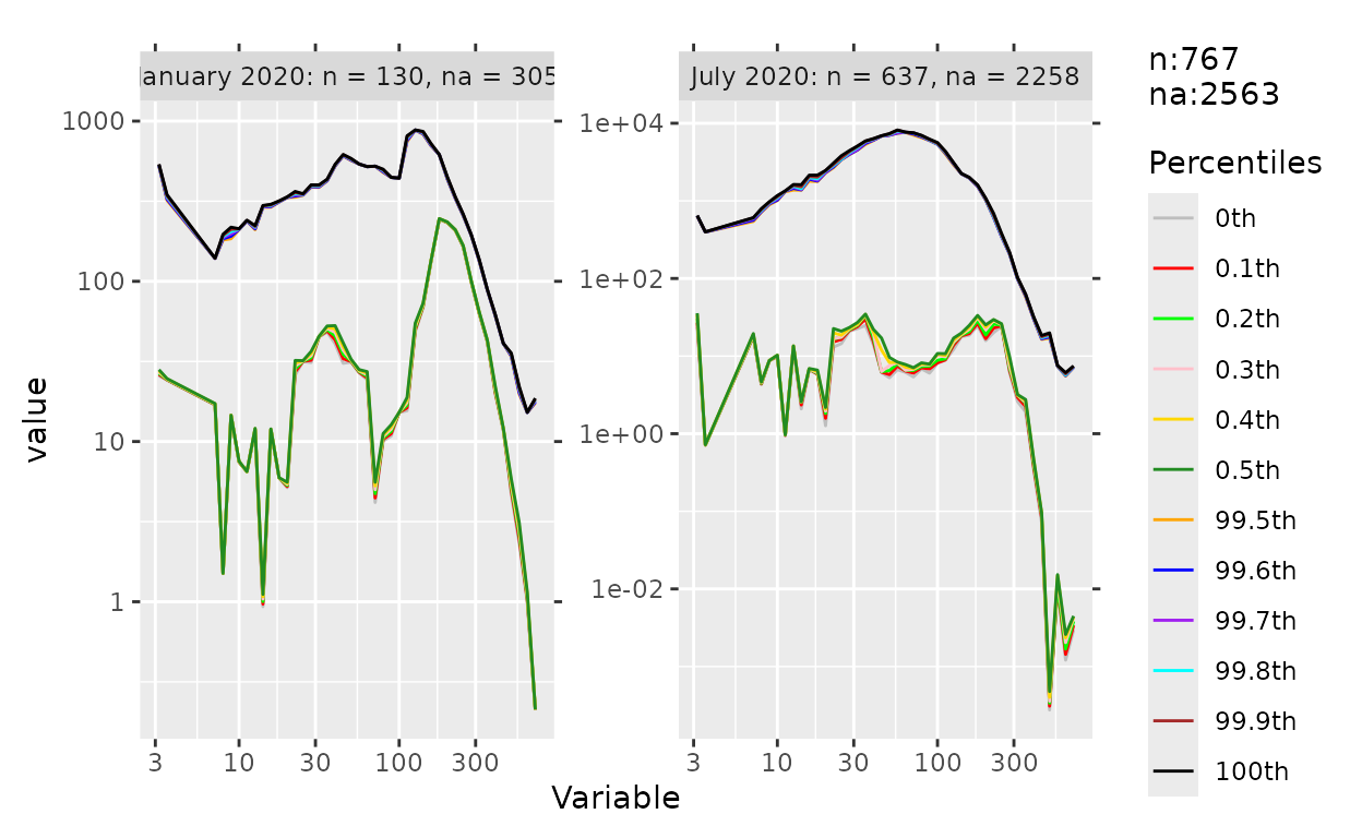

Compare with the earlier figure: the top and bottom percentile curves are smoother, the extreme tails are shorter, the interquartile band is tighter, and the number of missing values (na) is much smaller.

Step 4 — Short-period interpolation

step3 <- shorvalu(step2, cols = num_cols, cores = 1L)
sum(is.na(step2[, num_cols])) - sum(is.na(step3[, num_cols]))
#> [1] 2563

shorvalu fills remaining short gaps (within intervals = 30 minutes) from the nearest valid values. The remaining NAs are in gaps that are too long to interpolate. This is exactly why steps 1–3 must come first: after them, every NA that is left sits inside a short gap that has a valid anchor, so shorvalu can interpolate locally without crossing a long empty stretch.

Note that shorvalu() enforces this constraint on its own as well: it splits each series into short segments at every point where the gap between two adjacent observations exceeds intervals, and interpolates within each segment independently. The upstream obsedele() step and the internal segmentation are two complementary guarantees against the same failure mode. See the “When NOT to preprocess” section below for the full explanation.

One-call pipeline: `dataprep()`

For quick exploration the four steps are wrapped in a single call. We use the first 1,000 rows of data to keep the example fast.

demo <- data[1:1000, ]
res  <- dataprep(
  demo,
  cols     = size_bin_cols(demo),
  group    = 4,
  interval = 5,
  times    = 3,
  half     = 30,
  cores    = 1L
)
dim(res)
#> [1] 875  39

The arguments mirror the individual steps:

cols selects the numeric variables to process.
group selects the grouping column used by obsedele and condextr.
interval and times control how aggressively condextr marks outliers between two observation-deletion rounds.
fraction sets the missing-fraction cutoff for varidele.
half and by define the consecutive-missing window for obsedele.
intervals sets the maximum gap that shorvalu will fill.
cores controls the number of OpenMP threads used by the obsedele and condextr backends. NULL (default) lets each backend choose based on data size.

Inspecting the plan without running it

dry_run() actually runs varidele, obsedele, and detect_outliers on the input (in that order), but reports the effect on a copy and does not modify the caller’s data. It returns a list with per-step before/after counts, so it is a safe read-only operation.

report <- dry_run(
  data1,
  cols       = c("Nucleation", "Aitken", "Accumulation"),
  steps      = c("varidele", "obsedele", "outlier"),
  fraction   = 0.5
)
str(report, max.level = 2)
#> List of 7
#>  $ varidele     :List of 2
#>   ..$ removed_columns: chr(0) 
#>   ..$ removed_count  : int 0
#>  $ obsedele     :List of 3
#>   ..$ rows_before: int 7640
#>   ..$ rows_after : int 7640
#>   ..$ removed    : int 0
#>  $ outlier      :List of 3
#>   ..$ na_before: int 0
#>   ..$ na_after : int 1171
#>   ..$ added    : int 1171
#>  $ original_n   : int 7640
#>  $ original_ncol: int 7
#>  $ final_n      : int 7640
#>  $ final_ncol   : int 7

data1 is the aggregated seven-column table, so this example is read-only and fast.

Missing-value diagnostics

na_diagnose() is also read-only and works on any numeric table.

na_diagnose(data1, cols = 3:7)
#>       variable    n na na_frac na_runs max_run
#> 1   Nucleation 7640  0       0       0       0
#> 2       Aitken 7640  0       0       0       0
#> 3 Accumulation 7640  0       0       0       0
#> 4        tconc 7640  0       0       0       0
#> 5         TPNC 7640  0       0       0       0

Additional cleaning helpers

Function	Purpose
`detect_outliers()`	IQR / MAD / percentile masks
`winsorize()`	cap extreme values instead of removing them
`phys_filter()`	filter by physical bounds
`filter_high_cor()`	drop highly correlated variables
`filter_low_var()`	drop near-constant variables
`deduplicate()`	exact / fuzzy duplicate removal
`validate_data()`	rule-based validation
`balance_panel()`	balance an unbalanced panel

winsorize changes data, so we use a slice of data:

demo <- data[1:500, ]
head(winsorize(demo, cols = "7.94")[["7.94"]])
#> [1]  3.2424      NA 73.8825      NA  3.2418  6.4869

filter_low_var and filter_high_cor operate on any numeric table:

df <- data.frame(
  id    = 1:100,
  const = rep(5, 100),
  noise = rnorm(100, sd = 0.005)
)
names(filter_low_var(df, cutoff = 0.001))
#> [1] "id"

When NOT to preprocess

The pipeline above assumes that the input is high-resolution instrument data with intermittent gaps and occasional outliers. Three cases where the full pipeline is not appropriate:

Already-aggregated data. data1 is the seven-column aggregate of data. It has no long missing runs and no obvious outliers, so varidele, obsedele, condextr, and shorvalu have nothing to do.
Models that tolerate missing values. Gradient boosting, random forests, and XGBoost handle NA natively.
Gaps shorter than the physical mixing time. When the aerosol is well-mixed, a few missing points can be interpolated with negligible error. In that case, the observation-deletion step can be relaxed by increasing half.

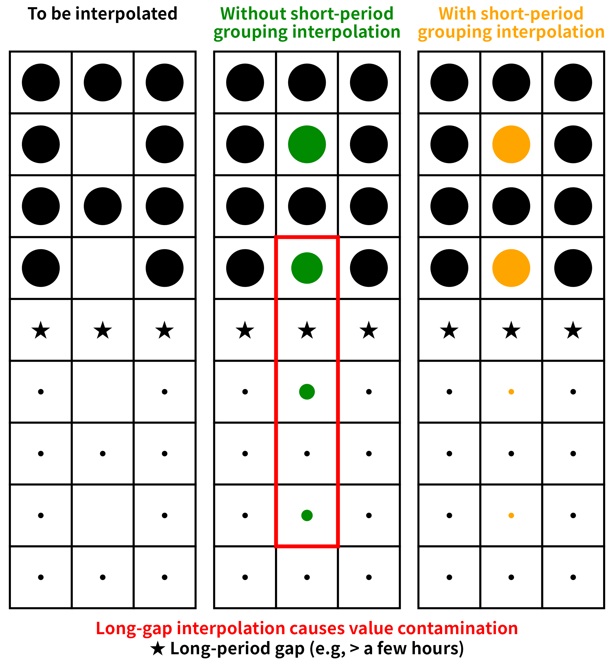
The figure below shows two complementary protections against the same failure mode: interpolating across a gap that is physically too long.

Upstream cleaning (varidele + obsedele). Before any interpolation runs, rows with long missing runs are deleted. After this step, every remaining NA sits inside a short gap that has a valid anchor within half minutes on at least one side. If this step were skipped, the values on either side of a long gap could belong to different physical regimes, and interpolating across the gap would produce a value that does not exist in nature.
Internal segmentation (shorvalu() itself). The interpolation function does not rely on the upstream step being complete. Before filling any NA, shorvalu() splits each series into short segments at every point where the time gap between two adjacent observations exceeds intervals (default 30 minutes), and interpolates within each segment independently. Even if a long gap survived the upstream cleaning — for example because the user relaxed half — shorvalu() would not bridge it: the segment boundary cuts the gap into two pieces, and each piece has to be interpolated from its own anchors.

The two protections are not redundant. The upstream cleaning is a preventive measure that preserves sample retention while bounding gap length; shorvalu()’s internal segmentation is a defensive measure that guarantees correctness regardless of upstream state. This is what “short-period grouping interpolation” means: interpolation is applied only where the value can be read from a nearby observation in the same segment.

Where to go next

Design philosophy and preprocessing methodology — vignette("dataprep-philosophy"). Why the pipeline has the shape it does, and how each step enforces a physical constraint.
Performance and cross-engine consistency — vignette("dataprep-performance"). Full benchmark tables (median + mean for every cell), the 8-engine consistency checks, and the reproducible runner.
Upgrading from 0.1.5 to 0.1.7 — vignette("dataprep-migration"). Behaviour changes, quantified effect on a real dataset, and a migration checklist.
Fast reshaping with melt() and dcast() — vignette("dataprep-melt-dcast").
Leakage-free preprocessing workflow — vignette("dataprep-workflow").

Session info

sessionInfo()
#> R version 4.6.1 (2026-06-24)
#> Platform: x86_64-pc-linux-gnu
#> Running under: Ubuntu 24.04.5 LTS
#> 
#> Matrix products: default
#> BLAS:   /usr/lib/x86_64-linux-gnu/openblas-pthread/libblas.so.3 
#> LAPACK: /usr/lib/x86_64-linux-gnu/openblas-pthread/libopenblasp-r0.3.26.so;  LAPACK version 3.12.0
#> 
#> locale:
#>  [1] LC_CTYPE=C.UTF-8       LC_NUMERIC=C           LC_TIME=C.UTF-8       
#>  [4] LC_COLLATE=C.UTF-8     LC_MONETARY=C.UTF-8    LC_MESSAGES=C.UTF-8   
#>  [7] LC_PAPER=C.UTF-8       LC_NAME=C              LC_ADDRESS=C          
#> [10] LC_TELEPHONE=C         LC_MEASUREMENT=C.UTF-8 LC_IDENTIFICATION=C   
#> 
#> time zone: UTC
#> tzcode source: system (glibc)
#> 
#> attached base packages:
#> [1] stats     graphics  grDevices utils     datasets  methods   base     
#> 
#> other attached packages:
#> [1] dataprep_0.1.7
#> 
#> loaded via a namespace (and not attached):
#>  [1] gtable_0.3.6       jsonlite_2.0.0     dplyr_1.2.1        compiler_4.6.1    
#>  [5] tidyselect_1.2.1   Rcpp_1.1.2         parallel_4.6.1     jquerylib_0.1.4   
#>  [9] systemfonts_1.3.2  scales_1.4.0       textshaping_1.0.5  yaml_2.3.12       
#> [13] fastmap_1.2.0      ggplot2_4.0.3      R6_2.6.1           generics_0.1.4    
#> [17] knitr_1.52         tibble_3.3.1       desc_1.4.3         bslib_0.12.0      
#> [21] pillar_1.11.1      RColorBrewer_1.1-3 rlang_1.3.0        cachem_1.1.0      
#> [25] xfun_0.61          fs_2.1.0           sass_0.4.10        S7_0.2.2          
#> [29] otel_0.2.0         cli_3.6.6          withr_3.0.3        pkgdown_2.2.1     
#> [33] magrittr_2.0.5     digest_0.6.39      grid_4.6.1         lifecycle_1.0.5   
#> [37] vctrs_0.7.3        evaluate_1.0.5     glue_1.8.1         farver_2.1.2      
#> [41] ragg_1.5.2         rmarkdown_2.32     tools_4.6.1        pkgconfig_2.0.3   
#> [45] htmltools_0.5.9